Explore Mecklenburg County on a map.

1. Prepare the datasets

Open the demo, select the Peter account if you have access, and open Query. Create a new editor tab so you keep your existing work. These queries use the account’s imported datasets; they do not require the collection agent.

For your own deployment, install Logship and import your CSV or TSV files with logsh. The table and column names below must match your imports. The datasets are not bundled with a fresh installation, and access to Peter is not granted by this tutorial.

Choose Execute after pasting this schema query. Check that the named columns exist before continuing:

$metadata.schema.tables.fields
| where TableName == "electiondata.votors.nc"
    or TableName == "parcels.nc.mecklenburg"
    or TableName == "addresses.nc"
| project TableName, ColumnName, ColumnType

Use DDLat and DDLong for geographic coordinates. The address dataset’s Lat and Long fields contain projected coordinates and are not suitable as map latitude and longitude.

2. Understand what is being matched

The sources format addresses differently. Voter addresses contain repeated spaces, parcel addresses include city and state, and the address dataset uses expanded suffixes such as STREET rather than ST.

The queries uppercase their join keys, remove spaces, and translate the address dataset’s street suffixes to common abbreviations. The geographic lookup produces one location per normalized address. Addresses with coordinate spreads greater than about 200 metres are excluded to avoid choosing between distant matches.

This is a deterministic matching example with partial coverage. Unit numbers, alternate spellings, unmatched suffixes, and incomplete addresses can leave records unmatched. Review match coverage before using the results for an analysis that needs complete counts.

3. Map matched registration records

Copy the complete query below into a new tab and choose Execute. When execution completes, select Render if the map has not opened automatically.

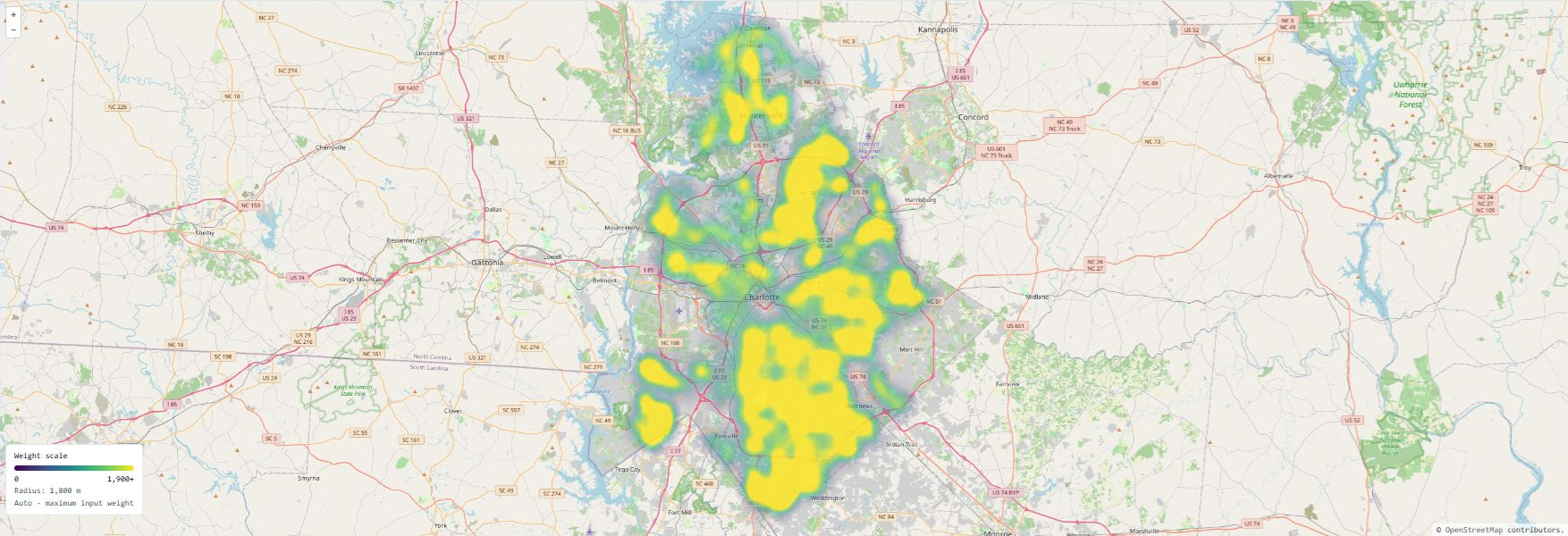
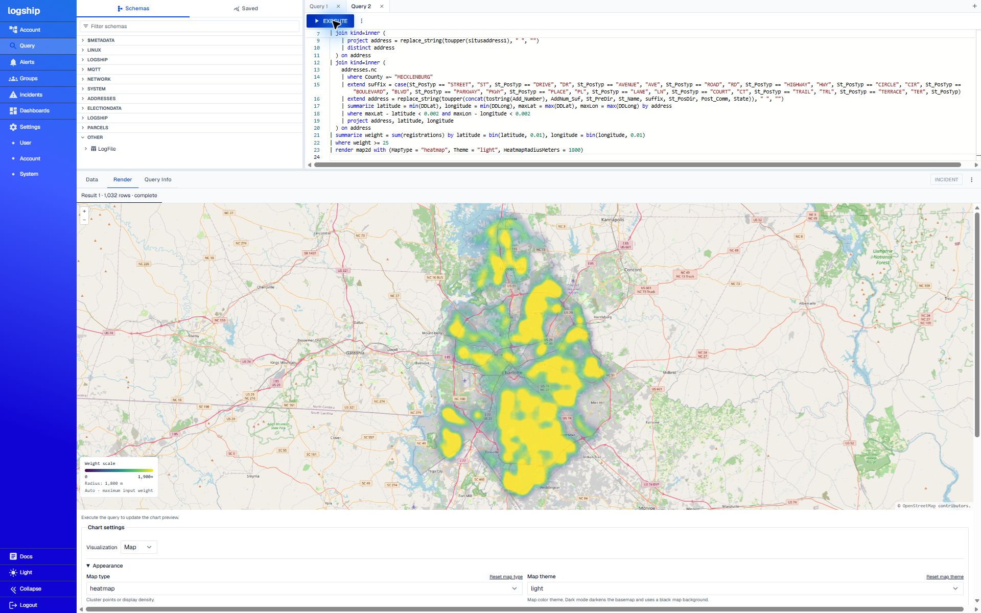
The query deduplicates registration ID/address pairs, matches them to distinct parcel addresses, and finds their geographic coordinates. It sums the matches in geographic cells of roughly 1 km and excludes cells with fewer than 25 matches.

View the complete query workspace

// Registration records matched to parcel addresses and geographic coordinates
electiondata.votors.nc
| where county_desc =~ "MECKLENBURG"
| project voter_reg_num, address = replace_string(toupper(concat(res_street_address, res_city_desc, state_cd)), " ", "")
| distinct voter_reg_num, address
| summarize registrations = count() by address
| join kind=inner (
    parcels.nc.mecklenburg
    | project address = replace_string(toupper(situsaddress1), " ", "")
    | distinct address
  ) on address
| join kind=inner (
    addresses.nc
    | where County =~ "MECKLENBURG"
    | extend suffix = case(St_PosTyp == "STREET", "ST", St_PosTyp == "DRIVE", "DR", St_PosTyp == "AVENUE", "AVE", St_PosTyp == "ROAD", "RD", St_PosTyp == "HIGHWAY", "HWY", St_PosTyp == "CIRCLE", "CIR", St_PosTyp == "BOULEVARD", "BLVD", St_PosTyp == "PARKWAY", "PKWY", St_PosTyp == "PLACE", "PL", St_PosTyp == "LANE", "LN", St_PosTyp == "COURT", "CT", St_PosTyp == "TRAIL", "TRL", St_PosTyp == "TERRACE", "TER", St_PosTyp)
    | extend address = replace_string(toupper(concat(tostring(Add_Number), AddNum_Suf, St_PreDir, St_Name, suffix, St_PosDir, Post_Comm, State)), " ", "")
    | summarize latitude = min(DDLat), longitude = min(DDLong), maxLat = max(DDLat), maxLon = max(DDLong) by address
    | where maxLat - latitude < 0.002 and maxLon - longitude < 0.002
    | project address, latitude, longitude
  ) on address
| summarize weight = sum(registrations) by latitude = bin(latitude, 0.01), longitude = bin(longitude, 0.01)
| where weight >= 25
| render map2d with (MapType = "heatmap", Theme = "light", HeatmapRadiusMeters = 1800)

Download the registration query

At validation on November 14, 2026: 1,032 cells and 474,885 matched registration records. Counts can change as source data changes. This map shows matched records, not voter turnout, party affiliation, total population, or proof that a person owns the matching property.

The 1,800-metre smoothing radius combines nearby counts into a density view. Brighter areas indicate concentrations of matching registrations.

4. Map median assessed residential values

Run the second query in another tab. It uses the parcel and address datasets, without the voter table. It selects one latest record per parcel, includes the listed single-family, townhouse, and condominium categories, and excludes non-positive assessed values.

View the complete query workspace

// Median assessed home value - USD per approximately 1 km cell
parcels.nc.mecklenburg
| where isnull(pid) == false
| extend address = replace_string(toupper(situsaddress1), " ", "")
| summarize value = argmax(timestamp, amt_totalvalue), propertyUse = argmax(timestamp, txt_propertyuse_desc), address = argmax(timestamp, address) by pid
| where value > 0
| where propertyUse == "SINGLE FAMILY RESIDENTIAL"
    or propertyUse == "SINGLE FAMILY RESIDENTIAL - ACREAGE"
    or propertyUse == "SINGLE FAMILY RESIDENTIAL - WATERFRONT"
    or propertyUse == "SINGLE FAMILY RESIDENTIAL - GOLF"
    or propertyUse == "TOWN HOUSE  SFR"
    or propertyUse == "CONDOMINIUM"
| join kind=inner (
    addresses.nc
    | where County =~ "MECKLENBURG"
    | extend suffix = case(
        St_PosTyp == "STREET", "ST", St_PosTyp == "DRIVE", "DR",
        St_PosTyp == "AVENUE", "AVE", St_PosTyp == "ROAD", "RD",
        St_PosTyp == "HIGHWAY", "HWY", St_PosTyp == "CIRCLE", "CIR",
        St_PosTyp == "BOULEVARD", "BLVD", St_PosTyp == "PARKWAY", "PKWY",
        St_PosTyp == "PLACE", "PL", St_PosTyp == "LANE", "LN",
        St_PosTyp == "COURT", "CT", St_PosTyp == "TRAIL", "TRL",
        St_PosTyp == "TERRACE", "TER", St_PosTyp)
    | extend address = replace_string(toupper(concat(tostring(Add_Number), AddNum_Suf, St_PreDir, St_Name, suffix, St_PosDir, Post_Comm, State)), " ", "")
    | summarize latitude = min(DDLat), longitude = min(DDLong), maxLat = max(DDLat), maxLon = max(DDLong) by address
    | where maxLat - latitude < 0.002 and maxLon - longitude < 0.002
    | project address, latitude, longitude
  ) on address
| extend northing = bin((latitude - 35.0) * 111.32, 1.0),
    easting = bin((longitude + 81.1) * 111.32 * cos(radians(35.25)), 1.0)
| summarize medianValue = percentile(value, 50.0), properties = count() by northing, easting
| where properties >= 10
| project latitude = 35.0 + (northing + 0.5) / 111.32,
    longitude = -81.1 + (easting + 0.5) / (111.32 * cos(radians(35.25))),
    medianValue, properties
| extend label = concat("$", tostring(bin(medianValue / 1000.0, 1.0)), "k | ", tostring(properties), " parcels")
| extend weight = medianValue
| render map2d with (
    MapType = "heatmap",
    Theme = "light",
    HeatmapMode = "geographic",
    HeatmapRadiusMeters = 450,
    HeatmapMaxWeight = 1500000)

Download the home-value query

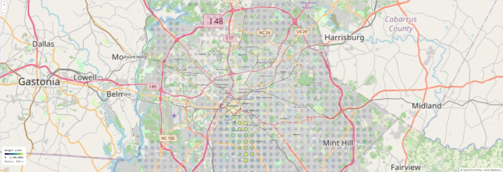
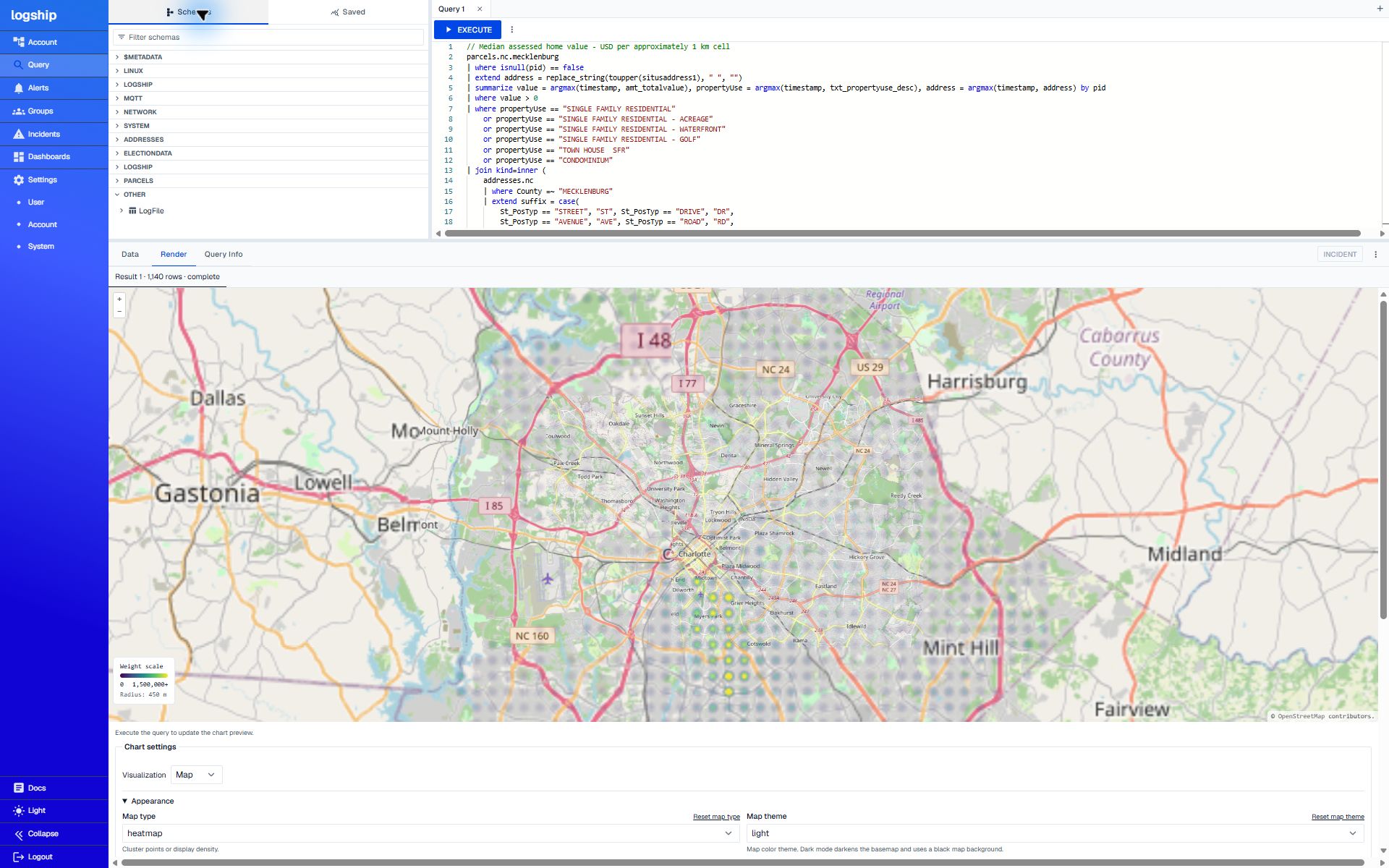
At validation: 1,140 cells containing 250,714 matched residential parcels. Each cell has at least 10 parcels. These are assessed values, not current market prices or recent sale prices.

Read the scale

The map’s Weight scale is in dollars because weight = medianValue. Its fixed range is $0 to $1,500,000+, with values above the maximum saturating the scale. Color at a cell’s center represents its median assessed value. The 450-metre radius keeps the hotspots of neighboring 1 km cells separate; color fades toward each hotspot’s edge.

The grid uses a local geographic approximation around latitude 35.25 degrees. It is suitable for this county-scale example. Cells omitted by the sample-size or matching filters are not zero-value areas.

Keep 50.0 in percentile(value, 50.0). It was validated for both odd and even sample sizes. The deployed version currently mishandles an integer percentile literal such as 50; that issue is tracked separately.

5. Save the maps in a dashboard

1. Open Dashboards in the same account and choose Create Dashboard.
2. Name it Mecklenburg data explorer. In edit mode, choose Add Chart.
3. Set Tile type to Kusto, paste one complete query, and save the chart.
4. Add a second Kusto chart for the other query. Give both maps enough space to keep the geographic detail and scale legible.
5. Choose Save on the dashboard, then reopen it from the dashboard list to confirm it persisted.

These examples intentionally analyze the imported snapshot rather than a recent time window. Avoid adding a short rolling timestamp filter unless you intend to restrict records by their ingestion timestamps.

Check the results